
First, if you have not read our previous post that used the Wolfram Model as a test, you might want to read that page.
In an effort to further explore the benefits of Numba we decided to use a new code that implements floating point operations. Here, we will compare the speeds of Numba, Python, and clever implementations of NumPy. We mostly followed the Julia set example from the book High Performance Python: Practical Performant Programming for Humans.
The Julia set algorithm:
- Create a 2D array with real numbers on the x-axis and imaginary numbers on the y-axis
- Iterate through the array and apply a function to each location. We used the function z2 + c where z was the complex number corresponding to the location in the array, and c is a complex constant.
- Keep doing this until a maximum number of iterations are reached, or the value of a location in the array gets too large.
- Plotting the absolute value of the array makes plots like those below.
Below, we include and compare four versions of the code:
- the raw Python
- NumPy
- NumPy with Numba’s jit
- Numba with njit, parallel=True
The raw Python takes a naive approach of iterating through an array and individually checking and calculating each location. The NumPy version uses NumPy operations to do this much more quickly.
Raw Python Code
Note that this uses loops.
This file contains hidden or bidirectional Unicode text that may be interpreted or compiled differently than what appears below. To review, open the file in an editor that reveals hidden Unicode characters.
Learn more about bidirectional Unicode characters
| import time #timing | |
| import numpy as np #arrays | |
| import numba as nb #speed | |
| x_dim = 1000 | |
| y_dim = 1000 | |
| x_min = -1.8 | |
| x_max = 1.8 | |
| y_min = -1.8j | |
| y_max = 1.8j | |
| z = np.zeros((y_dim,x_dim),dtype='complex128') | |
| for l in range(y_dim): | |
| z[l] = np.linspace(x_min,x_max,x_dim) -np.linspace(y_min,y_max,y_dim)[l] | |
| def julia_raw_python(c,z): | |
| it = 0 | |
| max_iter = 100 | |
| while(it < max_iter): | |
| #These will be expensive! | |
| for y in range(y_dim): | |
| for x in range(x_dim): | |
| if abs(z[y][x]) < 10: #Runaway condition | |
| z[y][x] = z[y][x]**2 + c #square and add c everywhere | |
| it += 1 | |
| return z | |
| start = time.perf_counter() | |
| julia_raw_python(-.4+.6j,z) #arbitrary choice of c | |
| end = time.perf_counter() | |
| print(end-start) |
Raw NumPy Code
Now, we use “clever” NumPy, rather than loops.
This file contains hidden or bidirectional Unicode text that may be interpreted or compiled differently than what appears below. To review, open the file in an editor that reveals hidden Unicode characters.
Learn more about bidirectional Unicode characters
| import time #timing | |
| import numpy as np #arrays | |
| import numba as nb #speed | |
| x_dim = 1000 | |
| y_dim = 1000 | |
| x_min = -1.8 | |
| x_max = 1.8 | |
| y_min = -1.8j | |
| y_max = 1.8j | |
| z = np.zeros((y_dim,x_dim),dtype='complex128') | |
| for l in range(y_dim): | |
| z[l] = np.linspace(x_min,x_max,x_dim) -np.linspace(y_min,y_max,y_dim)[l] | |
| def julia_numpy(c,z): | |
| it = 0 | |
| max_iter = 100 | |
| while(it < max_iter): | |
| z[np.absolute(z) < 10] = z[np.absolute(z) < 10]**2 + c #the logic in [] replaces our if statement. This line | |
| it += 1 #updates the whole matrix at once, no need for loops! | |
| return z | |
| start = time.perf_counter() | |
| julia_numpy(-.4+.6j,z) #arbitrary choice of c | |
| end = time.perf_counter() | |
| print(end-start) |
Python with njit and prange
Back to the loops, but adding Numba.
This file contains hidden or bidirectional Unicode text that may be interpreted or compiled differently than what appears below. To review, open the file in an editor that reveals hidden Unicode characters.
Learn more about bidirectional Unicode characters
| import time | |
| import numpy as np | |
| from numba import njit, prange | |
| x_dim = 1000 | |
| y_dim = 1000 | |
| x_min = -1.8 | |
| x_max = 1.8 | |
| y_min = -1.8j | |
| y_max = 1.8j | |
| z = np.zeros((y_dim,x_dim),dtype='complex128') | |
| for l in range(y_dim): | |
| z[l] = np.linspace(x_min,x_max,x_dim) -np.linspace(y_min,y_max,y_dim)[l] | |
| @njit(parallel = True) | |
| def julia_raw_python_numba(c,z): | |
| it = 0 | |
| max_iter = 100 | |
| while(it < max_iter): | |
| #These will be expensive! | |
| for y in prange(y_dim): #special loops for Numba! range -> prange | |
| for x in prange(x_dim): | |
| if abs(z[y][x]) < 10: #Runaway condition | |
| z[y][x] = z[y][x]**2 + c #square and add c everywhere | |
| it += 1 | |
| return z | |
| start = time.perf_counter() | |
| julia_raw_python_numba(-.4+.6j,z) | |
| end = time.perf_counter() | |
| print(end-start) |
Numpy with jit
Copy of “clever” NumPy, with Numba (jit).
This file contains hidden or bidirectional Unicode text that may be interpreted or compiled differently than what appears below. To review, open the file in an editor that reveals hidden Unicode characters.
Learn more about bidirectional Unicode characters
| import time | |
| import numpy as np | |
| from numba import jit | |
| x_dim = 1000 | |
| y_dim = 1000 | |
| x_min = -1.8 | |
| x_max = 1.8 | |
| y_min = -1.8j | |
| y_max = 1.8j | |
| z = np.zeros((y_dim,x_dim),dtype='complex128') | |
| for l in range(y_dim): | |
| z[l] = np.linspace(x_min,x_max,x_dim) -np.linspace(y_min,y_max,y_dim)[l] | |
| @jit() | |
| def julia_numpy_numba(c,z): | |
| it = 0 | |
| max_iter = 100 | |
| while(it < max_iter): | |
| z[np.absolute(z) < 10] = z[np.absolute(z) < 10]**2 + c #the logic in [] replaces our if statement. This line | |
| it += 1 #updates the whole matrix at once, no need for loops! | |
| return z | |
| start = time.perf_counter() | |
| julia_numpy_numba(-.4+.6j,z) | |
| end = time.perf_counter() | |
| print(end-start) |
We ran these codes on a desktop with:
- Xeon® Processor E5-1660 v4 (20M Cache, 3.2-3.6 GHz) 8C/16T 140W
- Linux CentOS
- 4*32GB 2Rx4 4G x 72-Bit PC4-2400 CL17 Registered w/Parity 288-Pin DIMM (128GB Total)
- 2*GeForce GTX 1080 Ti Founders Edition (PNY) 11GB GDDR5X – 960GB PM863a SATA 6Gb/s 2.5″ SSD, 1,366 TBW ( OS and Scratch ) 1.92TB PM863a SATA 6Gb/s 2.5″ SSD, 2,773 TBW
- RAVE Proprietary Liquid Cooling Kit
The times used in the graph below are the minimum times each code took for 100 trials to run with varying array sizes. (Size is the edge length of the Julia set.)
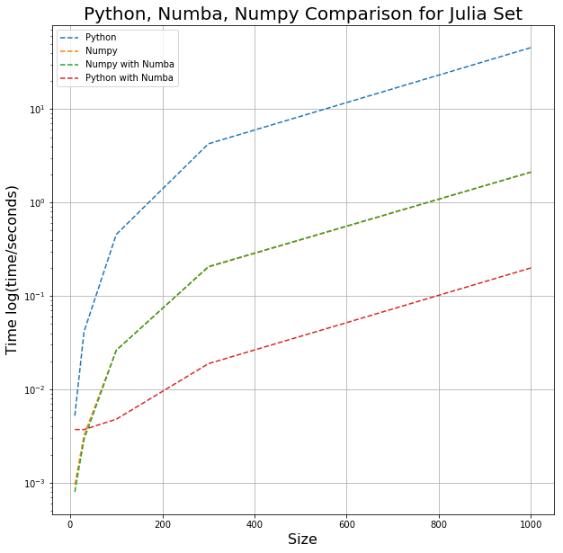
As you can see, using NumPy alone can speed up the Julia set calculation by a little over an order of magnitude; applying Numba to NumPy had no effect (as expected). Numba gave speeds 10x faster than the NumPy, illustrating the advantage Numba brings.
Credits:
Data:
All of the data produced can be found on David’s GitHub: https://github.com/DavidButts/Julia-Timing-Data